Netdata, Prometheus, Grafana Stack

In this blog, we will walk you through the basics of getting Netdata, Prometheus and Grafana all working together and monitoring your application servers. This article will be using docker on your local workstation. We will be working with docker in an ad-hoc way, launching containers that run /bin/bash and attaching a TTY to them. We use docker here in a purely academic fashion and do not condone running Netdata in a container. We pick this method so individuals without cloud accounts or access to VMs can try this out and for it’s speed of deployment.

Why Netdata, Prometheus, and Grafana

Some time ago I was introduced to Netdata by a coworker. We were attempting to troubleshoot python code which seemed to be bottlenecked. I was instantly impressed by the amount of metrics Netdata exposes to you. I quickly added Netdata to my set of go-to tools when troubleshooting systems performance.

Some time ago, even later, I was introduced to Prometheus. Prometheus is a monitoring application which flips the normal architecture around and polls rest endpoints for its metrics. This architectural change greatly simplifies and decreases the time necessary to begin monitoring your applications. Compared to current monitoring solutions the time spent on designing the infrastructure is greatly reduced. Running a single Prometheus server per application becomes feasible with the help of Grafana.

Grafana has been the go to graphing tool for… some time now. It’s awesome, anyone that has used it knows it’s awesome. We can point Grafana at Prometheus and use Prometheus as a data source. This allows a pretty simple overall monitoring architecture: Install Netdata on your application servers, point Prometheus at Netdata, and then point Grafana at Prometheus.

I’m omitting an important ingredient in this stack in order to keep this tutorial simple and that is service discovery. My personal preference is to use Consul. Prometheus can plug into consul and automatically begin to scrape new hosts that register a Netdata client with Consul.

At the end of this tutorial you will understand how each technology fits together to create a modern monitoring stack. This stack will offer you visibility into your application and systems performance.

Getting Started - Netdata

To begin let’s create our container which we will install Netdata on. We need to run a container, forward the necessary port that Netdata listens on, and attach a tty so we can interact with the bash shell on the container. But before we do this we want name resolution between the two containers to work. In order to accomplish this we will create a user-defined network and attach both containers to this network. The first command we should run is:

docker network create --driver bridge netdata-tutorial

With this user-defined network created we can now launch our container we will install Netdata on and point it to this network.

docker run -it --name netdata --hostname netdata --network=netdata-tutorial -p 19999:19999  centos:latest '/bin/bash'

This command creates an interactive tty session (-it), gives the container both a name in relation to the docker daemon and a hostname (this is so you know what container is which when working in the shells and docker maps hostname resolution to this container), forwards the local port 19999 to the container’s port 19999 (-p 19999:19999), sets the command to run (/bin/bash) and then chooses the base container images (centos:latest). After running this you should be sitting inside the shell of the container.

After we have entered the shell we can install Netdata. This process could not be easier. If you take a look at this link, the Netdata devs give us several one-liners to install Netdata. I have not had any issues with these one liners and their bootstrapping scripts so far (If you guys run into anything do share). Run the following command in your container.

wget -O /tmp/netdata-kickstart.sh https://my-netdata.io/kickstart.sh && sh /tmp/netdata-kickstart.sh --dont-wait

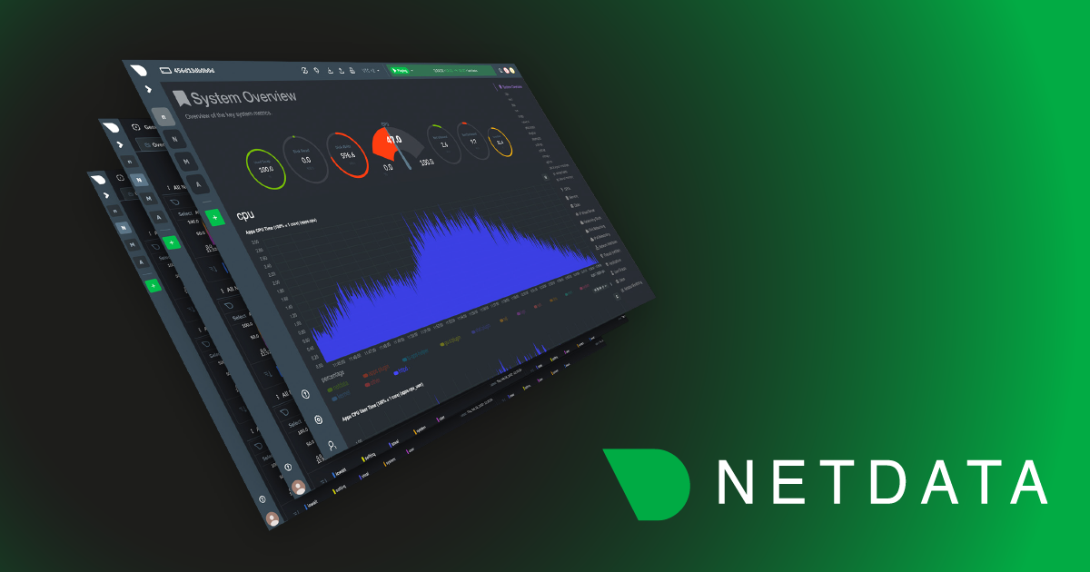
After the install completes you should be able to hit the Netdata dashboard at http://localhost:19999/ (replace localhost if you’re doing this on a VM or have the docker container hosted on a machine not on your local system). If this is your first time using Netdata I suggest you take a look around. The amount of time I’ve spent digging through /proc and calculating my own metrics has been greatly reduced by this tool. Take it all in.

Next I want to draw your attention to a particular endpoint. Navigate to http://localhost:19999/api/v1/allmetrics?format=prometheus&help=yes In your browser. This is the endpoint which publishes all the metrics in a format which Prometheus understands. Let’s take a look at one of these metrics. netdata_disk_space_GiB_average{chart="disk_space._run",dimension="avail",family="/run",mount_point="/run",filesystem="tmpfs",mount_root="/"} 0.0298195 1684951093000 This metric is representing several things which I will go in more details in the section on Prometheus. For now understand that this metric: netdata_disk_space_GiB_average has several labels: (chart, family, dimension, mountt_point, filesystem, mount_root). This corresponds with disk space you see on the Netdata dashboard.

This CHART is called system.cpu, The FAMILY is cpu, and the DIMENSION we are observing is system. You can begin to draw links between the charts in Netdata to the Prometheus metrics format in this manner.

Prometheus

We will be installing Prometheus in a container for purpose of demonstration. While Prometheus does have an official container I would like to walk through the install process and setup on a fresh container. This will allow anyone reading to migrate this tutorial to a VM or Server of any sort.

Let’s start another container in the same fashion as we did the Netdata container.

docker run -it --name prometheus --hostname prometheus \
--network=netdata-tutorial -p 9090:9090  centos:latest '/bin/bash'

This should drop you into a shell once again. Once there quickly install your favorite editor as we will be editing files later in this tutorial.

yum install vim -y

You will also need wget and curl to download files and sudo if you are not root.

yum install curl sudo wget -y

Prometheus provides a tarball of their latest stable versions here.

Let’s download the latest version and install into your container.

cd /tmp && curl -s https://api.github.com/repos/prometheus/prometheus/releases/latest \
| grep "browser_download_url.*linux-amd64.tar.gz" \
| cut -d '"' -f 4 \
| wget -qi -

mkdir /opt/prometheus

sudo tar -xvf /tmp/prometheus-*linux-amd64.tar.gz -C /opt/prometheus --strip=1

This should get Prometheus installed into the container. Let’s test that we can run Prometheus and connect to it’s web interface.

/opt/prometheus/prometheus --config.file=/opt/prometheus/prometheus.yml

Now attempt to go to http://localhost:9090/. You should be presented with the Prometheus homepage. This is a good point to talk about Prometheus’s data model which can be viewed here: https://prometheus.io/docs/concepts/data_model/ As explained we have two key elements in Prometheus metrics. We have the metric and its labels. Labels allow for granularity between metrics. Let’s use our previous example to further explain.

netdata_disk_space_GiB_average{chart="disk_space._run",dimension="avail",family="/run",mount_point="/run",filesystem="tmpfs",mount_root="/"} 0.0298195 1684951093000

Here our metric is netdata_disk_space_GiB_average and our common labels are chart, family, and dimension. The last two values constitute the actual metric value for the metric type (gauge, counter, etc…). We also have specific label for this chart named mount_point,filesystem, and mount_root. We can begin graphing system metrics with this information, but first we need to hook up Prometheus to poll Netdata stats.

Let’s move our attention to Prometheus’s configuration. Prometheus gets it config from the file located (in our example) at /opt/prometheus/prometheus.yml. I won’t spend an extensive amount of time going over the configuration values documented here: https://prometheus.io/docs/operating/configuration/. We will be adding a new job under the scrape_configs. Let’s make the scrape_configs section look like this (we can use the DNS name Netdata due to the custom user-defined network we created in docker beforehand).

scrape_configs:
  # The job name is added as a label `job=<job_name>` to any timeseries scraped from this config.
  - job_name: 'prometheus'

    # metrics_path defaults to '/metrics'
    # scheme defaults to 'http'.

    static_configs:
      - targets: ['localhost:9090']

  - job_name: 'netdata'

    metrics_path: /api/v1/allmetrics
    params:
      format: [ prometheus ]

    static_configs:
      - targets: ['netdata:19999']

Let’s start Prometheus once again by running /opt/prometheus/prometheus. If we now navigate to Prometheus at http://localhost:9090/targets we should see our target being successfully scraped. If we now go back to the Prometheus’s homepage and begin to type netdata\_ Prometheus should auto complete metrics it is now scraping.

Let’s now start exploring how we can graph some metrics. Back in our Netdata container lets get the CPU spinning with a pointless busy loop. On the shell do the following:

[root@netdata /]# while true; do echo "HOT HOT HOT CPU"; done

Our Netdata cpu graph should be showing some activity. Let’s represent this in Prometheus. In order to do this let’s keep our metrics page open for reference: http://localhost:19999/api/v1/allmetrics?format=prometheus&help=yes. We are setting out to graph the data in the CPU chart so let’s search for system.cpu in the metrics page above. We come across a section of metrics with the first comments # COMMENT homogeneous chart "system.cpu", context "system.cpu", family "cpu", units "percentage" followed by the metrics. This is a good start now let us drill down to the specific metric we would like to graph.

# COMMENT
netdata_system_cpu_percentage_average: dimension "system", value is percentage, gauge, dt 1501275951 to 1501275951 inclusive
netdata_system_cpu_percentage_average{chart="system.cpu",family="cpu",dimension="system"} 0.0000000 1501275951000

Here we learn that the metric name we care about is netdata_system_cpu_percentage_average so throw this into Prometheus and see what we get. We should see something similar to this (I shut off my busy loop)

This is a good step toward what we want. Also make note that Prometheus will tag on an instance label for us which corresponds to our statically defined job in the configuration file. This allows us to tailor our queries to specific instances. Now we need to isolate the dimension we want in our query. To do this let us refine the query slightly. Let’s query the dimension also. Place this into our query text box. netdata_system_cpu_percentage_average{dimension="system"} We now wind up with the following graph.

Awesome, this is exactly what we wanted. If you haven’t caught on yet we can emulate entire charts from Netdata by using the chart dimension. If you’d like you can combine the chart and instance dimension to create per-instance charts. Let’s give this a try: netdata_system_cpu_percentage_average{chart="system.cpu", instance="netdata:19999"}

This is the basics of using Prometheus to query Netdata. I’d advise everyone at this point to read this page. The key point here is that Netdata can export metrics from its internal DB or can send metrics as-collected by specifying the source=as-collected URL parameter like so. http://localhost:19999/api/v1/allmetrics?format=prometheus&help=yes&types=yes&source=as-collected If you choose to use this method you will need to use Prometheus’s set of functions here: https://prometheus.io/docs/querying/functions/ to obtain useful metrics as you are now dealing with raw counters from the system. For example you will have to use the irate() function over a counter to get that metric’s rate per second. If your graphing needs are met by using the metrics returned by Netdata’s internal database (not specifying any source= URL parameter) then use that. If you find limitations then consider re-writing your queries using the raw data and using Prometheus functions to get the desired chart.

Grafana

Finally we make it to grafana. This is the easiest part in my opinion. This time we will actually run the official grafana docker container as all configuration we need to do is done via the GUI. Let’s run the following command:

docker run -i -p 3000:3000 --network=netdata-tutorial grafana/grafana

This will get grafana running at http://localhost:3000/. Let’s go there and login using the credentials Admin:Admin.

The first thing we want to do is click “Add data source”. Let’s make it look like the following screenshot

With this completed let’s graph! Create a new Dashboard by clicking on the top left Grafana Icon and create a new graph in that dashboard. Fill in the query like we did above and save.

Conclusion

There you have it, a complete systems monitoring stack which is very easy to deploy. From here I would begin to understand how Prometheus and a service discovery mechanism such as Consul can play together nicely. My current prod deployments automatically register Netdata services into Consul and Prometheus automatically begins to scrape them. Once achieved you do not have to think about the monitoring system until Prometheus cannot keep up with your scale. Once this happens there are options presented in the Prometheus documentation for solving this. Hope this was helpful, happy monitoring.

• prometheus
• exporter
• grafana
• netdata
• monitoring-stack